The Use of Generative Adversarial Networks in Medical Image Segmentation

Edition dos of me ripping off my uni work

Dec 04, 2023

Ello

Generative adversarial networks (GANs) are very cool and so I picked them to write a literature review about for university. This is a more little known application but you might’ve heard of text-to-image translation like Midjourney. You’ve definitely heard of ChatGPT, it is responsible for thousands of Desmonds across UK universities in the last couple of years. You might wonder how they work, and I’m not going to tell you in much detail because this is a lit review. But I tried to pitch a few concepts in an understandable way whilst glossing over complex details that I don’t really understand well either to be honest. Some of the maths doesn’t format well here, email me for the full pdf

Also, I start my first placement today in radiotherapy, wish me luck.

Abstract

Medical image segmentation plays a pivotal role in computer-aided diagnosis and treatment with its invaluable insights into pathological conditions. This literature review explores the application of generative adversarial networks in the realm of medical image segmentation, assessing how different types of networks can be paired with a specific task for precise segmentation. This ranges from retinal vessel segmentation employing conditional GANs to brain tumor delineation using cycleGANs and liver segmentation via Wasserstein GANs. Moreover, the review addresses the significance of automated segmentation, highlighting the diagnostic accuracy improvements in comparison to traditional segmentation networks, and the potential for enhanced patient outcomes. However, this review also examines the limitations, including interpretability issues, dataset constraints, and class imbalances, which hinder widespread clinical adoption at the time of writing.

Glossary of Abbreviations

GAN: Generative Adversarial Network

CAD: Computer Aided Diagnosis

MRI: Magnetic Resonance Imaging

CT: Computed Tomography

CNN: Convolutional Neural Network

AI: Artificial intelligence

ML: Machine Learning

ROI: Region Of Interest

G: Generator

D: Discriminator

Purpose and Aims

This review is written with the aim of explaining the background and operating principles of generative adversarial networks before evaluating how such nets can be used in the medical imaging segmentation space. This review also looks to discuss the challenges that researchers have faced in their applications and what the future holds for programs that utilise generative adversarial networks in a GAN-based medical image segmentation workflow. The review is divided into the following sections:

1. Introduction

2. Generative Adversarial Network Background and Operating Principles

3. GAN Models and Architectures used in Medical Image Segmentation

4. Summary and Future Work

1 Introduction

Computer aided diagnosis (CAD) tools greatly aid healthcare professionals in the interpretation of medical images. It requires dedicated multi-disciplinary input from the areas of radiology, pathology, computer vision and image processing, and machine learning/ artificial intelligence. More automated systems are developed to improve the efficiency of diagnosis and treatment processes, resulting in more positive patient outcomes and experiences. This can manifest as shorter scanning times due to faster acquisition, earlier detection of disease, and more accurate diagnosis and classification, empowering patients with more detailed analysis of their images and facilitating more active patient participation in their pathway. This aligns with the NHS’ Long Term Plan where personalised healthcare is due to play a large part in improving the effectiveness of the service, reaching 2.5 million people in 2024 with the aim of doubling that within a decade [1].

A main component of computer aided diagnosis is segmentation. Segmentation is the sectioning of images into meaningful regions, this could be a tumour, blood vessels, or a whole organ depending on the task. By finding the borders of regions of interest, one is able to perform many important processes, from diagnosis and quantitative analysis to treatment planning and monitoring. Segmentation can of course be done manually, with radiologists or well-trained clinical image analysts tracing by hand on medical images to contour regions of interest. This is very time-consuming and expensive from a labour cost and effective use of time perspective, especially regarding 3D images in which the ’segmenter’ has to trace over many slices to obtain a volume, making the process a ripe opportunity when considering implementing automated workflows.

Generative adversarial networks are a machine learning technique that create synthetic data that resembles training data, in this case medical image segmentations. They have the advantage of being able to function both supervised and unsupervised depending on their fine structure, meaning that large labelled datasets can be utilised in supervised architectures but the scarcity of large labelled datasets for certain segmentation tasks doesn’t negatively affect unsupervised learning flows. These approaches can be balanced with semi-supervised method in which auxiliary data is fed into the network to aid accurate data generation.

2 Generative Adversarial Networks: Background and Operating Principles

2.1 Background and General Theory of GANs

This section lines out the short history of generative adversarial networks and goes through how they work to transform an input of random noise into a realistic imposter that even experienced professionals are sometimes unable to catch out. A core aim of deep learning is to create complex models that represent probability distributions of input data such that they can be mapped to simple class labels, with the ability to generalise algorithms to accept input data of many types. Generative adversarial networks are a class of deep learning algorithm introduced in 2014 by Ian Goodfellow that are inspired by the concept of a ’zero sum game’ from Game Theory, where in a game of two players, one agent’s gain is the other’s loss (and vice versa) [2]. In the case of GANs, the two competing adversaries are sub-models known as Generators (G) and Discriminators (D). The generator typically takes in random noise and transforms it to create a plausible example of data such as a medical image which are fed into the discriminator, which is a binary classifier and assigns its input as either ’real’ or ’fake’. In effect, the generator is trying to trick the discriminator into classifying its output data as real. Figure 1 shows how the sub-models interact with one another in the original proposed architecture from 2014, being used to detect handwritten digits from the famous MNIST dataset [3]. The output of the discriminator decides the penalty, or loss, of each sub-model, in which a back-propagation mechanism is used to update the weights of each network.

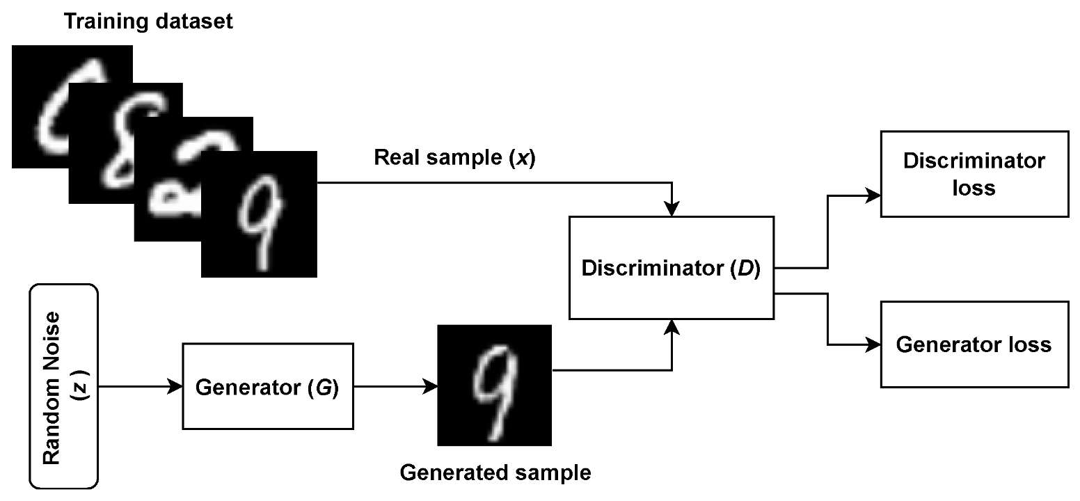
Figure 1: The original generative adversarial network architecture being used to classify handwritten digits [3].

2.2 Training the Network

The final aim of GANs training for the generator to produce fake data with a high enough quality such that the discriminator has a detection accuracy of 50%, this is known as convergence. Despite being a desired end state of training, in the original network it is a transient state rather a stable one. When the network is over-trained past this point of convergence, the discriminator is essentially flipping a coin to classify data. This results in the discriminator potentially providing junk feedback to the generator, reducing the quality of its output. As previously mentioned, loss functions are used to communicate weight updates for both the generator and discriminator. These can come in many forms depending on the tailored task but the most simple and first introduced one is the minimax loss. Taken from Game Theory, the minimax loss function has a solution known as the Nash equilibrium, which is a stable state in which neither agent can improve their performance (Equation 1). The function maps the distance between probability distributions of the generated and real data, this is known as cross-entropy [4].

min G max D V (D, G) = Ex[log ((D(x))] + Ez[log (1 − (D(G(z))] (1)

Where:

V : The value function.

Ex: Expected value over all real data instances.

D(x): The estimate from the discriminator of the probability that real data instance x is real.

Ez: The expected vale over all fake data instances (from G(z))

D(G(z)): The probability, according to the discriminator that a fake instance is real.

3 GAN Models and Architectures used in Medical Image Segmentation

There are many GAN architectures being designed to perform tailored segmentation tasks, with modified loss functions and even non-random generator inputs being introduced. This section is broken down into sub-sections of anatomical regions and how pairing a specific kind of generative adversarial network architecture works when given the task. The hierarchy of various GAN architectures is shown in Figure 2 for reference in the discussion of some of the variations present in this review.

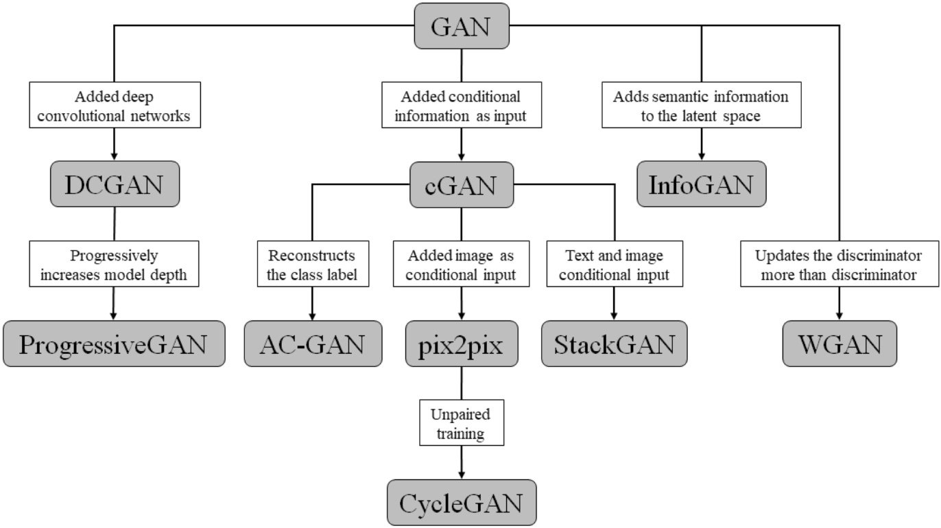
Figure 2: Hierarchy of different generative adversarial network architectures [5].

3.1 Retina Vessel Segmentation with a Conditional Generative Adversarial Network (cGAN)

Fundoscopic images are visualisations of the retina that can provide rich information regarding the eye and even the general health of the patient. Images help to diagnose conditions such as retina vein collusion and artery collusion as well as hypertension and diabetes by detecting abnormalities in the retina’s blood vessels. In order to do this, segmentation of the vascular architecture of the retina is essential in visualising and quantifying the vessels. Son et al. (2019) proposed a framework called RetinaGAN, based off of a conditional GAN network (cGAN) [6]. In this network type, additional information is fed to the generator and discriminator in the training phase, known as conditional variables. This could be class labels or even data from other modalities. Equation 2 shows how the value function varies from the original loss function in Equation 1 with the introduction of auxiliary information, y. In this case, it was the addition of ’gold standard’ manually segmented data, otherwise known as ’ground truths’.

min G max D V (D, G) = Ex[log ((D(x|y))] + Ez[log (1 − (D(G(zy))] (2)

So y is presented as a generator input in a joint hidden representation as shown in Figure 3, taken from the original paper that introduced conditional adversarial networks [7]. RetinaGAN boasted an improved segmentation of fine vessels in comparison to typical convolutional neural networks such as U-Net that were not equipped with a discriminator. This was because the pixel values around fine vessels don’t differ much making them easily missed at the start of training in comparison to thick branches. The U-Net is only punished by segmentation loss, which is a very small loss due to the fine vessels not consisting of many pixels. On the other hand, the cGAN is penalised for missing fine vessels that are included in the gold standard, meaning that over time the cGAN performed much better than the U-Net in this respect as shown in Figure 4. These fine structures are important in fundoscopy when evaluating a patient’s visual acuity, especially in the case of diabetic macular edema, where swelling in the eye can cause vision loss. This method of conditional GAN usage needs larger datasets of gold standard labelled data to improve and to be extended to other similar uses such as optic disc segmentation for glaucoma detection and treatment. This optic disc segmentation was tried but was outperformed significantly by the U-Net due to its conspicuity. Another criticism of this method is the long length of the training phase. The generator and discriminator were trained in an alternating function, one being trained for a set number of epochs before switching to the other and so on. This naturally takes around double the time to train the model than training both sub-models simultaneously as is done in the original generative adversarial network and in many other architectures of the GAN hierarchy.

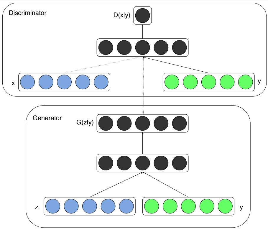
Figure 3: The conditional adversarial net [7].

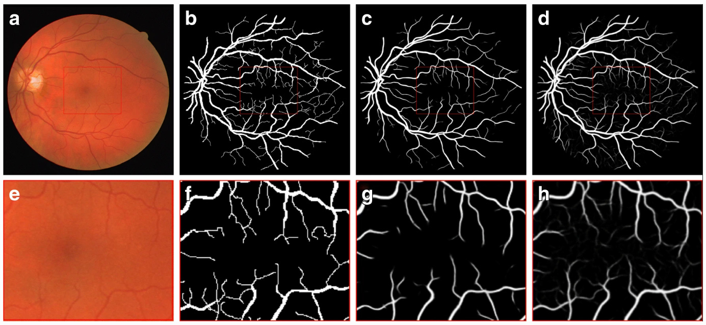
Figure 4: Fundus image (a, e), gold standard (b, f), output of U-Net (c, g), and output of RetinaGAN-Image (d, h). Central area of images at the top row is zoomed up at the bottom row [6].

3.2 Brain Tumour Segmentation with a Cycle Generative Adversarial Network (cycleGAN)

Gliomas are the most malignant brain tumours in adults and occur with highly variable prognoses and severity, defined by the World Health Organisation into ’grades’. Finding the borders of the tumour accurately is important for treatment planning for surgery and radiotherapy, so doctors can precisely know the location and size of it. An automated model would also aid in monitoring the progression of the tumour and its responsiveness to treatment. In such a high risk area as the brain, precise segmentation is absolutely crucial in the potential clinical feasibility of an automatic brain tumour segmentation program.

Nema et al., (2020) introduced RescueNET, an unpaired network that didn’t rely on the mass generation of labelled brain tumours from radiologists, circumventing the issue of a lack of labelled data that limits the training of supervised networks [8]. This was done by modifying cycleGAN, which has recently become a very popular type of generative adversarial network since its inception in 2017 [9].

Where the initial Goodfellow GAN takes random noise as the only generator input, the cycleconsistent GAN takes an image as the input, eliminating the need for paired data whilst translating images from a source domain, such as a brain image, to a target domain such as a brain image with the tumour segmented. This image-to-image translation differs from the basic GAN not only from its input but also in the design and function. CycleGANs use two generators and two discriminators to facilitate the inclusion of cycle-consistency loss, which is a key feature of such nets and adds to the normal adversarial loss, giving more precise parameter updates and sometimes accounting for vanishing gradients.

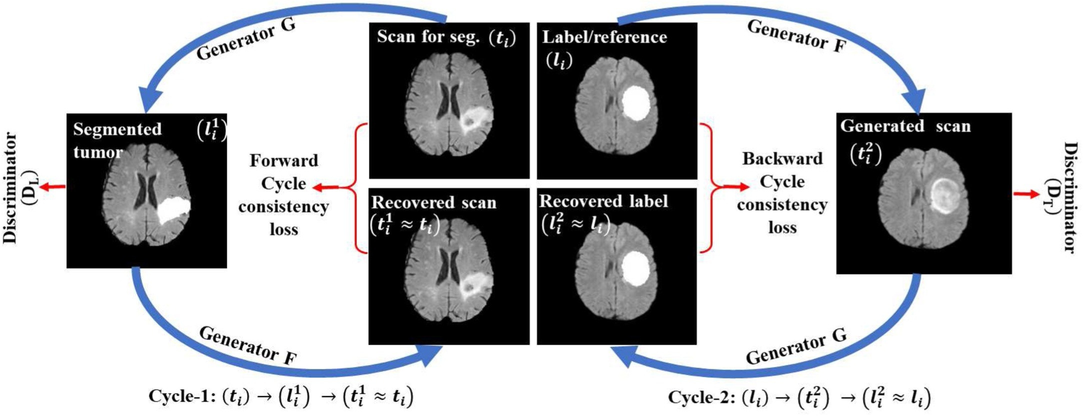
Figure 5: The unpaired training procedure for RescueNET [8].

From Figure 5 the cyclic flow of the GAN can be seen. Two generators (G and F) are trained simultaneously with the two discriminators (DT and DL). In the first cycle (cycle 1) the network G generates a tumour segmentation l 1 i from input image ti and then the network F generator uses this to recover a similar image (t 1 i ) to the input ti . the second cycle (cycle 2) performs in a similar manner as the first, using the F generator to produce a scan t 2 1 and G to produce the labelled image l 2 i which is similar to the reference label li . Then we move onto the discriminators. Discriminator DT is used to discriminate between the input scan ti and the generated scan t 2 i whilst the discriminator DL aims to distinguish between the reference label li and the image with the generated tumour segmentation l 1 i [8].

The results of using unpaired networks in a cyclic fashion produced encouraging segmentation results, getting a higher region overlap (dice score) than the other methods of U-Net and ResNET, shown in Figure 7. The evaluation method of dice similarity score is a simple but effective metric when comparing an automatically segmented image with ground truth labels and is defined in Equation 3, where TP, FP, and FN correspond to pixels that are true positives, false positives, and false negatives respectively.

DICE = 2 × T P / (T P + F P) + (T P + F N) (3)

The proposed method gave dice similarity scores in the 90% range when test on the BraTS 2015 dataset, beating out all of the other state of the art non-GAN methods. Despite being a good metric for obtaining a general idea, for a brain tumour a more advanced border comparison metric would’ve been more suitable, as it is crucial that the exact borders of the generated segmentation is as close to the ground truth as possible. A boundary loss function and associated evaluation metric could be added to this model for this [10].

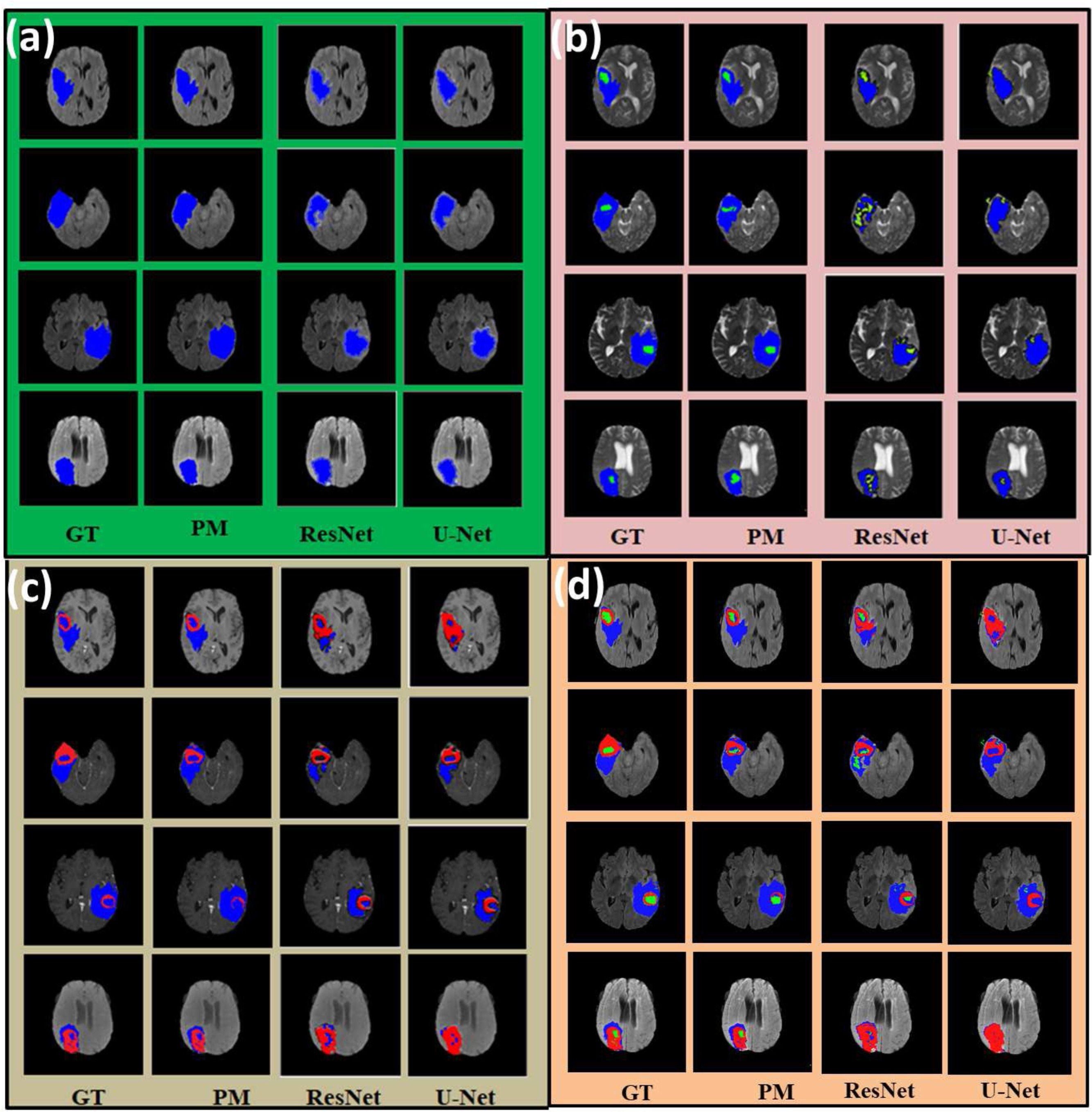
Figure 6: Segmentation results from brain MRI images, showing the ground truth (GT) when compared to the proposed method of RescueNET (PM), Res-Net, and U-Net. ”(a) Result of whole tumor segmentation on FLAIR MRI scan. (b) Result of whole and core tumor segmentation on T2 MRI scan. (c) Result of whole and enhance tumor segmentation on T1c MRI scan. (d) Combined result on FLAIR MRI scan. Note: Blue, Red and Green color shows the whole, enhance and core tumor region respectively” [8].

This sort of network showed promising performance to in future possibly be generalised to brain tumour segmentation tasks from other image types, with a multi-modality learning system potentially providing even greater accuracy in locating and sectioning brain tumours. Training on multiple image modalities would take a far more complex net, considering the differences between even different image types in the same modality such as T1 and T2 weighted images in MRI are significant.

3.3 Liver Segmentation with a Wasserstein Generative Adversarial Network (WGAN)

Liver segmentation is a step in liver disease diagnosis and a worthwhile exercise when considering treatment and surgery planning, and prognosis. It is typically a difficult task to automate liver segmentations due to large variability between individuals, the complexity of the anatomical structure of the liver, and its close proximity to surrounding organs and tissues that can cause interference such as the gallbladder. Ma et al., (2021) expanded the capability of previous work to segment the liver with a generative adversarial structure [11]. A so called Wasserstein GAN (WGAN) was used in this instance which differs from the original net structure greatly in an attempt to remedy the vanishing gradient issue where gradients that are used to update the parameters of the generator and discriminator are too small to make a difference over long training periods. This makes the WGAN more stable in training, encouraging more a more efficient convergence process [12]. This indicator used as the loss function in a WGAN is known as the Wasserstein or earth mover distance; it measures the distance between distributions of data in the training dataset and those observed in the generated set (Equation 4). A VNet network was also implemented on the generator side for segmentation which differs from past methods but is beyond the scope of this review.

min G max D V (D, G) = Ex[D(x)] + Ez[D(G(z))] (4)

In short, the WGAN moves away from the discriminator predicting whether an image is real towards the concept of a critical model that scores the fakeness or realness of a given image. So instead of a discriminator, there is a critic that trains the generator. The change to the earth mover distance also facilitates constant improvement of the net, which differs from the discriminator model whose useful updates dwindle once trained. Using the mathematical concept of the popular ’dice’ evaluation coefficient, a dice loss can was used on the generator side by calculating similarity between generated and ground truth segmentations. Equation 5 shows the dice loss function where A is the set of predicted foreground pixels and B is the set of real foreground pixels.

L_Dice = 1 − 2|A ∩ B|/ |A| + |B| = |A| − |A ∩ B| + |B| − |A ∩ B| / |A| + |B| (5)

When tested on the CHAOS and LiTS liver CT datasets, dice scores of over 90% were produced, over a 3% improvement from other methods (Figure 7). However, the loss function was deemed unsuitable for other tasks such as lung nodule detection and brain tumour segmentation. The limited scope of the application of this algorithm makes it less attractive for clinicians than a theoretical general, one-stop-shop model framework for which many applications are effectively possible.

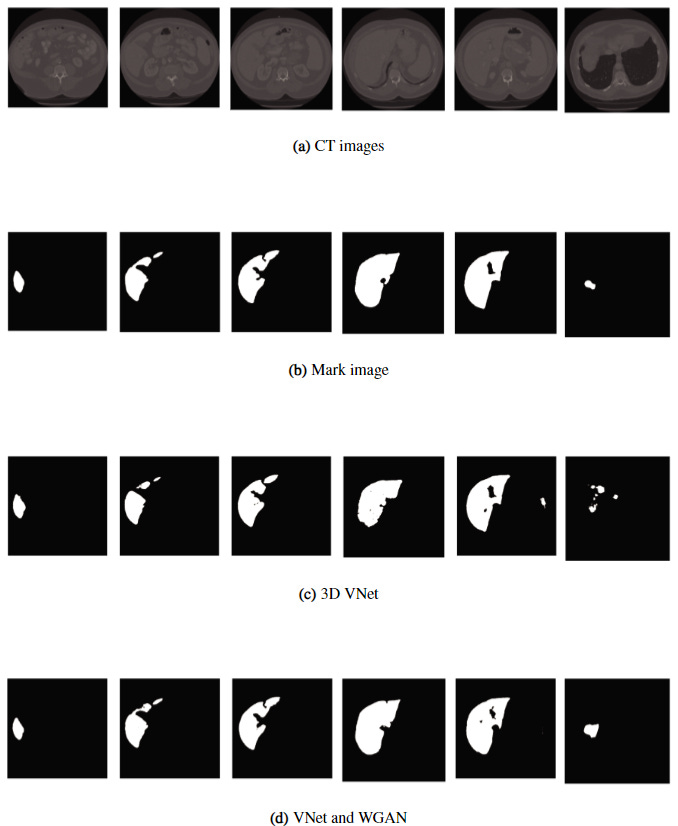
Figure 7: Comparison of results between the 3D VNet and the proposed method (bottom) [11].

4 Summary and Future Work

Through the tweaking and tailoring of the revolutionary base concept of generative adversarial networks, many groups have been successful in the task of medical image segmentation, with the aim of producing accurate enough models to be used clinically in more automated workflows and improving patient outcomes, experiences, and personalised treatment. This review has shown how Game Theoretic models of a zero sum game can be used for a number of segmentation tasks but lack the generality for a single network to be able to applied across anatomical regions and image modalities. By being a complex class of system, a large drawback is the interpretability of GANs. They are known for their ’black box’-like nature and so may not yet be trusted by clinical staff that don’t have a deep knowledge base surrounding artificial intelligence and machine learning. Supervised GANs systems, like any supervised medical image networks, suffer from the the lack of labelled data for which supervised ML algorithms require masses of. It’s not just the size of labelled datasets which is an issue, there is also a large class imbalance in training data where rare diseases and abnormalities are underrepresented in sets. Future work based on the current research gaps of class imbalance, data availability, interpretability, and potential ethical considerations could help to propel GAN-based medical image segmentation into widespread clinical use once solved.

maklito

Discussion about this post

References

[1] H. Alderwick and J. Dixon, “The nhs long term plan,” 2019.
[2] I. Goodfellow, J. Pouget-Abadie, M. Mirza, B. Xu, D. Warde-Farley, S. Ozair, A. Courville, and Y. Bengio, “Generative adversarial nets,” Advances in neural information processing systems, vol. 27, 2014.
[3] K. Saleh, S. Sz´en´asi, and Z. V´amossy, “Generative adversarial network for overcoming occlusion in images: A survey,” Algorithms, vol. 16, no. 3, p. 175, 2023.
[4] T. Salimans, I. Goodfellow, W. Zaremba, V. Cheung, A. Radford, and X. Chen, “Improved techniques for training gans,” Advances in neural information processing systems, vol. 29, 2016.
[5] J. J. Jeong, A. Tariq, T. Adejumo, H. Trivedi, J. W. Gichoya, and I. Banerjee, “Systematic review of generative adversarial networks (gans) for medical image classification and segmentation,” Journal of Digital Imaging, vol. 35, no. 2, pp. 137–152, 2022.
[6] J. Son, S. J. Park, and K.-H. Jung, “Towards accurate segmentation of retinal vessels and the optic disc in fundoscopic images with generative adversarial networks,” Journal of digital imaging, vol. 32, no. 3, pp. 499–512, 2019.
[7] M. Mirza and S. Osindero, “Conditional generative adversarial nets,” arXiv preprint arXiv:1411.1784, 2014.
[8] S. Nema, A. Dudhane, S. Murala, and S. Naidu, “Rescuenet: An unpaired gan for brain tumor segmentation,” Biomedical Signal Processing and Control, vol. 55, p. 101641, 2020.
[9] J.-Y. Zhu, T. Park, P. Isola, and A. A. Efros, “Unpaired image-to-image translation using cycle-consistent adversarial networks,” in Proceedings of the IEEE international conference on computer vision, pp. 2223–2232, 2017.
[10] H. Kervadec, J. Bouchtiba, C. Desrosiers, E. Granger, J. Dolz, and I. B. Ayed, “Boundary loss for highly unbalanced segmentation,” in International conference on medical imaging with deep learning, pp. 285–296, PMLR, 2019.
[11] J. Ma, Y. Deng, Z. Ma, K. Mao, and Y. Chen, “A liver segmentation method based on the fusion of vnet and wgan,” Computational and Mathematical Methods in Medicine, vol. 2021, pp. 1–12, 2021.
[12] M. Arjovsky, S. Chintala, and L. Bottou, “Wasserstein generative adversarial networks,” in International conference on machine learning, pp. 214–223, PMLR, 2017. 10